Hello, if you have any need, please feel free to consult us, this is my wechat: wx91due
DEPARTMENT OF STATISTICS AND ACTUARIAL SCIENCE
STAT3600 Linear Statistical Analysis
Chapter 5 Analysis of Variance
5 Analysis of Variance
5.1 Sum of Squares
Recall that the fitted (predicted) value of a regression model is given by:

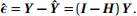
with residuals
In the following, different types of sum of squares are defined:
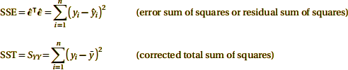
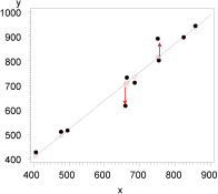
The error sum of squares (SSE) is the variation around the regression line. Use SLR as illustra-tion. Graphically,
The regression model would have a good fit if the residuals εˆi ’s are small. Thus, SSE provides a measure of the goodness of fit of the model. If we had ignored the explanatary variables in the regression model and fitted a fixed constant to the response (i.e. assumed that the responses constitute an i.i.d. constant sample), then the residual sum of square becomes SY Y (= SST).
Evidently, SST ≥ SSE. It can be shown that their difference, namely SST−SSE = SSR, where SSR can also be expressed as sum of squares,
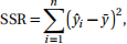
which is called regression sum of squares.
This difference measures how effective X (the p explanatory or predictor variables) is to ex-plain the variation in the response Y and that a large value in SSR corresponds to significant predictors of the response variable Y .
An analysis of variance is a formal method for determining whether SSR is large enough for concluding that the fitted regression model is useful in explaining the variation in the re-sponse Y . This method is based on the fact that the total variability of response is the sum of the variability explained by model and the unexplained variability:
SST = SSR+SSE
The above stated definitions can be summarized by the so called ANOVA (ANalysisOfVAriance) table below. Proofs will be provided in Section 5.2.
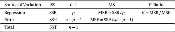
Features of ANOVA table:
• bottom item = sum of items above;
• each sum of squares (SS) accounts for a source of variation in Y ;
• each SS is associated with a degree of freedom (d. f.);
• mean square (MS) = SS/d. f.;
• The ratio of Regression Mean Square and Error Mean Square, the so called F -ratio.
5.2 F Test for Regression Relation
To test whether there is a regression relation between the dependent variable Y and the set of X variables, set the hypotheses as
H0 : β1 = β2 = ... = βp = 0 vs. H1 : not all βj equal to zero.
Recall that the hat matrix is defined as

Let

Hence, we have
I = A1 + A2 + A3.
It can be shown that Aj for j = 1, 2, 3 are idempotent, i.e.  Also
Also

and
tr (A2) = tr (H) − tr (A) = p.
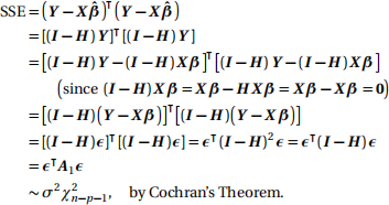
Under the general hypothesis H1 that not all βj equal to 0:
Y − X β = ε ∼ Nn (0,σ2 I).
Recall the properties of the hat matrix that H X = X and (I −H)2 = I −H , so
Also note the following expansion:
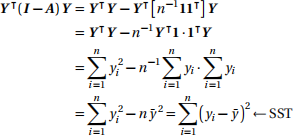
Thus, SST can be written in matrix notation as
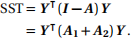
Hence, SSR becomes
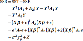
where Z is a normal random variable with mean 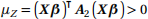 and variance
If H0 is true, it can be shown that the normal variable Z becomes zero. By Cochran’s Theorem,

are independent. As a result, the test statistic is the F -ratio as given in the ANOVA table:
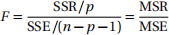
is Fp,n−p−1 distributed underH0 . We rejectthenullhypothesisH0 iff F > Fα,p,n−p−1 for 100(α)% level of significance.
A large value of the F-ratio is the result of a large value in SSR that contributes much to SST, that means X (the p explanatory variables) is effective in explaining the variation in Y . On the other hand, a small F -ratio is the result of a small value of SSR that contributes little to SST , that implies X is not very effective in explaining the variation in Y .
Physical interpretation of H0 and H1 :
For H0 , it means {X1 ,...,Xp } collectively is NOT effective in explaining the response (Y 0 s) variation.
For H1 , it means {X1 ,...,Xp } collectively is effective in explaining the response (Y 0 s) vari-ation.
The test assesses only “collective” effects of {X1 ,...,Xp } as a group, but not as individual factors.