Hello, if you have any need, please feel free to consult us, this is my wechat: wx91due
DEPARTMENT OF STATISTICS AND ACTUARIAL SCIENCE
STAT3600 Linear Statistical Analysis
Chapter 4 Multiple Linear Regression
4 Multiple Linear Regression
4.1 Model Formulation and Assumptions
A sample of n observations is observed in the form of (yi , xi 1 ,..., xi p ) for the ith observation:
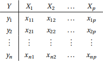
where Y is the response variable and X1 ,...,Xp are the explanatory variables. A multiple linear regression model (MLR) assumes:
(A1) X1 ,...,Xp are non-random variables or they are given,
(A2) yi = β0 + β1 xi 1 + ... + βp xi p + εi with εi ∼ N (0, σ2),
(A3) the responses y1 ,..., yn are independent.
Equivalently, in matrix form,

where,
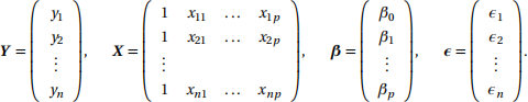
β0 ,β1 ,...βp are the unknown regression coefficients with βj measuring the associated effect of X j on Y ; and X is an n × (p + 1) design matrix with known entries. Here we assume the columns of X are linearly independent. The word ’linear’ in a linear model refers to the prop-erty that E (Y ) is ‘linear’ in the regression coefficients β0 ,β1 ,...βp , but not necessarily in each explanatory variable.
Examples:
Linear models (linear combination of parameters):
• y = β0 + β1 x + ε (SLR)
• y = β0 + β1 x + β2x2 + ε
(explanatory variables: x1 = x , x2 = x2)
• y = β0 + β1 sin 2πz1 − β2 log z2 + ε
(explanatory variables: x1 = sin 2πz1, x2 = −log z2)
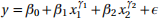
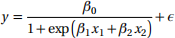
NOT Linear models:
• 
• 
4.2 Model Fitting by Least Square Method
Same as the SLR, the unknown parameters β can be estimated by minimizing the Error Sum of Squares or Sum of the Squared Errors given the observed data of the explanatory variable X and response variable Y.
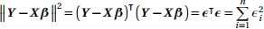
Hence,
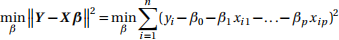
The LS-estimator ˆβ = [ˆβ0, ˆβ1 ,...,ˆβp]T satisfies
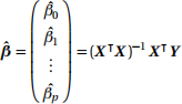
which is the result we obtained for the SLR in Chapter 3.
4.2.1 Example (Environmental Data)
A data set is taken from an environmental study that measured four variables:
ozone (Y ) - ozone surface concentration in New York, in parts per million;
radiation (X1) - solar radiation, in langley;
temperature (X2) - observed temperature, in degrees Fahrenheit;
wind (X3) - wind speed, in miles per hour;
for 30 days.
Table 1: Environmental data
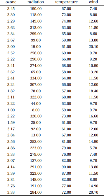
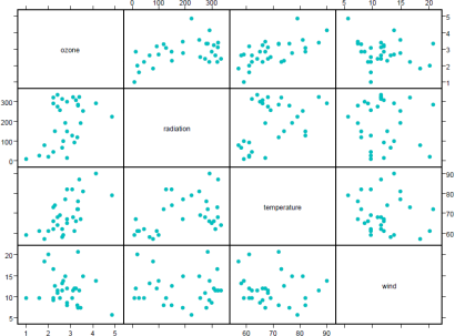
Figure 1: Scatterplot matrix for the environmental data
Multiple regression of Y on X1, X2 and X3:
yi = β0 + β1 xi 1 + β2 xi 2 + β3 xi 3 + εi or Y = X β + ε (matrix form),
where
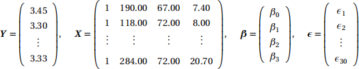
and
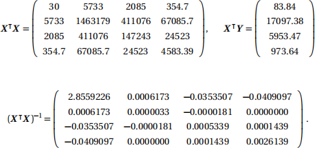
As a result, the LS-estimate of β is:
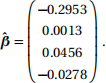
Hence, the fitted model is given by:

When other factors are fixed, on average, ozone
• increases by 0.0013 parts per million when radiation increases by 1 langley.
• increases by 0.0456 parts per million when temperature increase by 1 degree Fahren-heit.
• decreases by 0.0278 parts per million when wind increases by 1 mile per hour.
4.2.2 Example (Philadelphia Birth Data)
These are data based on a 5% sample of all births occurring in Philadelphia in 1990. The sample has 1115 observations (after deleting 32 cases with incomplete information) on five variables:
grams (Y ) - Birth weight in grams;
ethnic (X1 ) - Mother is African American (1=yes, 0=no);
educ (X2 ) - Mother’s years of education (0-17 Years);
smoke (X3 ) - Whether mother smoked during pregnancy (1=yes, 0=no);
gestate (X4 ) - Gestational age in weeks;
Multiple regression of Y on X1, X2, X3 and X4:
yi = β0 + β1 xi 1 + β2 xi 2 + β3 xi 3 + β4 xi 4 + εi or Y = X β + ε (matrix form),
where
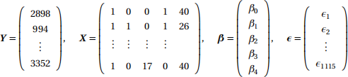
and
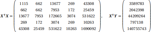
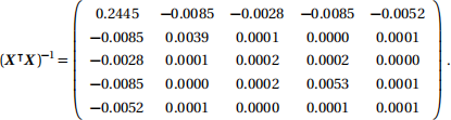
As a result, the LS-estimate of β is:
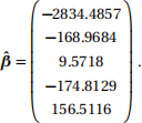
Hence, the fitted model is given by:

When other factors are fixed, on average, the weight of the child
• decreases by 168.9684 grams when the mother is Afro-American.
• increases by 9.5718 grams when the education duration of the mother increases by 1 year.
• decreases by 174.8129 grams when the mother is a smoker.
• increases by 156.5116 grams when the gestational age increases by 1 week.