MA513
Homework #1
Due date: Thursday, December 28
1.2 What is a time series?Explain the meaning of trend effects,seasonal variations,and random error.
1.13 Discuss the potential difficulties of forecasting the daily closing price of a specific stock on the New York Stock Exchange.Would the problem be different (harder,easier)if you were asked to forecast the closing price of a group of stocks,all in the same industry(say, the pharmaceutical industry)?
2.35 Consider an N-span moving average where each observation is weighted by a constant,say,a;≥0.Therefore the weighted moving average at the end of period T is

a.Why would you consider using a weighted moving average?
b.Show that the variance of the weighted moving average is Var 
2.36 Consider the Hanning filter.This is a weighted moving average.
a.Find the variance of the weighted moving average for the Hanning
filter.Is this variance smaller than the variance of a simple span-3 moving average with equal weights?
5.For a time series data set with 100 observations.Y₂ =1.76440, =0.85559 and r,=0.62805.Then rs =
For an approximation of the standard error of rs if the time series is white noise,we have se(rs)≥ ·
3.1 An article in the journal Air and Waste (Update on Ozone Trends in California's South Coast Air Basin,Vol.43,1993)investigated the ozone levels in the South Coast Air Basin of California for the years 1976-1991.The author believes that the number of days the ozone levels exceeded 0.20 ppm(the response)depends on the seasonal meteorological index,which is the seasonal average 850-millibar Temperature (the predictor).Table E3.1 gives the data.
a. Construct a scatter diagram of the data.
b. Estimate the prediction equation.
c.Test for significance of regression.
d. Calculate the 95%CI and PI on for a seasonal meteorological index value of 17.Interpret these quantities.
e.Analyze the residuals.Is there evidence of model inadequacy? f.Is there any evidence of autocorrelation in the residuals?

3.22 Analyze the regression model in Exercise 3.1 for leverage and influ- ence.Discuss your results.
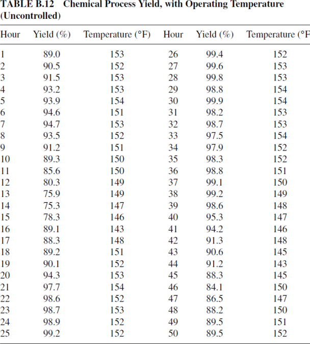
3.10 Table B.13 in Appendix B contains hourly yield measurements from a chemical process and the process operating temperature.Fit a regression model to these data,using the temperature as the pre- dictor.Analyze the residuals from this model.Is there evidence of autocorrelation in these data?

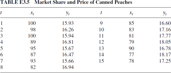
3.11 The data in Table E3.5 give the percentage share of market of a particular brand of canned peaches (y,)for the past 15 months and the relative selling price(x,).

a. Fit a simple linear regression model to these data.Plot the resid- uals versus time.Is there any indication of autocorrelation?
b. Use the Durbin-Watson test to determine if there is positive autocorrelation in the errors.What are your conclusions?
c .Use one iteration of the Cochrane-Orcutt procedure to estimate the regression coefficients.Find the standard errors of these regression coefficients.
d. Is there positive autocorrelation remaining after the first itera- tion?Would you conclude that the iterative parameter estimation technique has been successful?
3.28 Table B.10 in Appendix B presents monthly data on airline miles flown in the United Kingdom.Fit an appropriate regression model to
these data.Analyze the residuals and comment on model adequacy.
