Power System Operation and Control

Aim: To be able to carry out basic MATLAB calculations for small-signal stability analysis

Entering State-Space Models into MATLAB

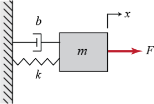
Now we will show you how to enter the state space equations into am-file MATLAB. Consider a Mass-Spring-Damper system as shown below:

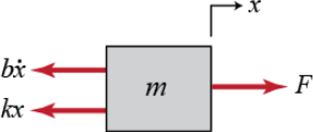
The free body diagram for this system is:

From the diagram the state space equations can be written as follows:

If we are interested in controlling the position of the mass, then the output equation is as follows:

Now create anew m-file and enter the following commands

m = 1;

k = 1;

b = 0.2;

F = 1;

A = [0 1; -k/m -b/m];

B = [0 1/m]';

C = [1 0];

D = [0];

sys = ss(A,B,C,D)

The output will looks like:

a =

x1    x2

x1     0     1

x2    - 1  -0.2

b =

u1

x1   0

x2   1

c =

x1  x2

y1   1   0

d =

u1

y1   0

Continuous-time model.

Entering Transfer Function Models into MATLAB

Now we will show you how to enter transfer functions of the above mass-spring- damper system into MATLAB.

Enter the following commands into them-file:

s = tf('s');

sys = 1/(m*s^2+b*s+k)

Sometimes you may need to define the transfer function model using the numerator and denominator polynomial coefficients directly rather than using the symbolic s variable:

num = [1];

den = [m b k];

sys = tf(num,den)

The results of both methods will be the same:

Transfer function:

1

s^2 + 0.2 s + 1

Stability

The transfer function is especially useful when analysing the system stability. The location of poles is an indication for the stability of the system.

The following MATLAB commands can be entered to find out the location of poles

s = tf('s');

G = 1/(s^2+2*s+5)

pole(G)

Transfer function:

1

s^2 + 2 s + 5

ans =

- 1.0000 + 2.0000i

- 1.0000 - 2.0000i

Thus we can tell that the system is stable since the real parts of the poles are both negative.

The stability of a system may also be found from the state-space representation. The eig command can be used to calculate the eigenvalues:

[A,B,C,D] = ssdata(G);

eig(A)

The same results will appear.

First order systems

In order to analyse a first order system the step response and bode plot are normally used.

See following command:

k_dc = 5;

Tc = 10;

u = 2;

s = tf('s');

G = k_dc/(Tc*s+1)

step(u*G)

bode(G)

Then the step response and bode plot of the system transfer function will be shown as follows:

By right click on the step response graph and select Characteristics, you can choose to have several system matrices overlaid on the response: settling time, rise time, etc..

Second order systems

For the second order systems the pole zero map will be used to illustrate the system dynamic behaviour:

k_dc = 1;

w_n = 10;

zeta = 0.2;

s = tf('s');

G1 = k_dc*w_n^2/(s^2 + 2*zeta*w_n*s + w_n^2);

pzmap(G1)

axis([-3 1 -15 15])

Root locus analysis

First of all we will learn how to plot the root locus of a transfer function. Consider the system described by the following transfer function:

The root locus can be plotted by the following commands:

s = tf('s');

sys = (s + 7)/(s*(s + 5)*(s + 15)*(s + 20));

rlocus(sys)

axis([-22 3 -15 15])