Hello, if you have any need, please feel free to consult us, this is my wechat: wx91due

DEPARTMENT OF STATISTICS AND ACTUARIAL SCIENCE

STAT3600 Linear Statistical Analysis

Chapter 3 Simple Linear Regression

3 Simple Linear Regression

3.1 Motivation

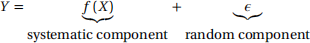
In many situations, the value taken by one variable Y is influenced by or related to the value taken by some other variable X. In this chapter, we are mainly interested in determining what relationship exists between Y (dependent variable, response) and one X (independent vari- able, covariate, explanatory variable) (for example, Yi is the monthly expenditure of the i-th person while Xi is monthly income of the same person). We wish to describe the relationship between X and Y by means of a mathematical formula (or mathematical model) given by

Y = f (X )

However, even if the model is true, our data will not agree perfectly with the model in general. Unlike in some physical science subjects where there may be exact functional rela- tionships between variables while in economics and most other fields, the functional rela- tionships are usually not exact. We express our model as

3.2 Model Formulation and Assumptions

When the data are of the form (x1, y1) , . . ., (xn, yn) (with one dependent and one independent variable only), the simplest form is the simple linear regression model (SLR) given by

Yi = β0+ β 1xi + ε i , i = 1,2, . . . , n

where β 's are the regression parameters, ε i's are stochastic disturbances or random errors which are not observable. Moreover we assume that the values of X1,..., Xn are non-random, i.e. fixed or regarded as given.

After collection of the data, the first thing to do should be plotting the data points on a scatter diagram. Suppose the scatter diagram suggests a linear relationship between X and Y or a linear relationship is suggested by the subject matter knowledge or scientific evidence, we may approach to fit a simple linear regression model of the form

Assumptions

(A1)  E (Ei) = 0 that implies E ( Y j X = xi) = β0+β1xi (primary assumption);

(A2)  Var (Ei) = σ2  (constant variance);

(A3)  The E i’s are uncorrelated (uncorrelatedness).

3.3 Least Square Estimator

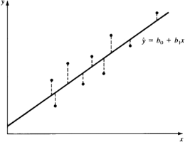
The unknown parameters are β0, β1, and σ2. The parameters β0 and β1 are called the inter- cept and slope, respectively and are termed regression coefficients. Determination of the best fit line or the estimation of β0  and β 1  from the observed data cannot be performed without specification of the criterion. The most commonly used criterion is to minimize the Sum of the Squared Errors (SSE), which is the sum of square of the vertical deviations from the fitted straight line. Mathematically, we have

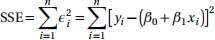
where yi is the observed value of Yi .  Our objective is to choose β0  and β1 to minimize SSE, and this method is known as the method of least squares (LS).

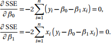
On differentiating SSE with respect to β0and β 1 and set to zero, we have the normalequa- tions:

Solving for β0 and β1, we obtain the LS -estimator

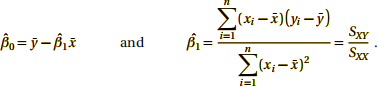
Note that the estimators are linear in yi’s. The following figure illustrates the application of the least square method on a single linear regression:

3.3.1 Example (Westwood Company Data)

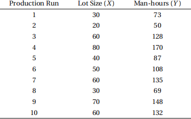
Let man-hours be the dependent variable Y and lot size be the independent variable X. The simple linear regression model is given by

man-hours = β0+β 1lot size+ ε

The least square estimate of β0and β 1 are therefore

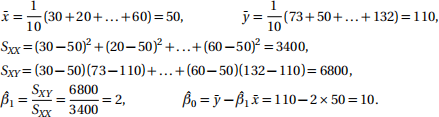
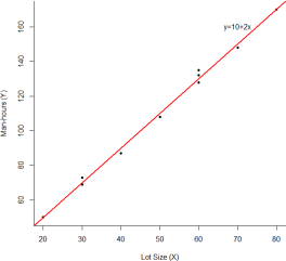
Hence, the estimated regression line is given by:

man-hours = 10 + 2 × lot size.

3.3.2 Example (Cholesterol Data)

The data are put in pairs as follows

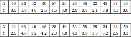
Let the plasma levels of total cholesterol (in mg/ml) be the dependent variable Y and the ages be the independent variable X. The simple linear regression model is given by

cholesterol levels = β0+β1ages + ε

The least square estimate of β0and β 1 are therefore

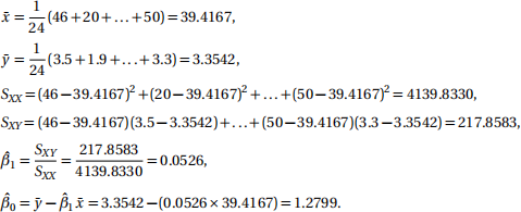
Hence, the estimated regression line is given by:

cholesterol levels = 1.2799 + 0.0526 × ages.