STAT GR 5241–Practice Final
Problem 1 (20 points, 5 points each)
Please answer the following questions.
(a) Can the number of nodes in a tree classifier be larger than the number of features in the data used to train that tree?
(b) Is a classifier trained on more training data more likely to overfit?
(c) Given a sample ˜(x) 1’··· ’˜(x)n and an estimator S(ˆ), we have described in class how a bootstrap estimator S(ˆ)BS can be computed based on B bootstrap samples. This idea is also used in the bagging algorithm. What is the advantage of the bootstrap estimator over the original estimator? Please explain briefly.
(d) Assume that the data x1’x2’··· ’xn aregenerated from a one-dimensional Gaussian distribution with mean μ and variance 1. Assume that the prior distribution of μ is a one dimensional Gaussian distribution with mean 2 and variance 1. The maximum a posteriori (MAP) estimator for μ can be expressed as
ˆ(μ)MAP = argmaxμ ∈R{φ(x1’x2’··· ’xn ;μ)}
for some function φ(x1’x2’··· ’xn ;μ) of x1’x2’··· ’xn and μ . Please write down the explicit form of φ(x1’x2’··· ’xn ;μ) (which should not involve any integral).
Hint: The density of a one-dimensional Gaussian distribution with mean μ and variance σ2 is given by

Problem 2 (30 points, 7.5 points each)
Please answer the following questions on tree-based classifiers.
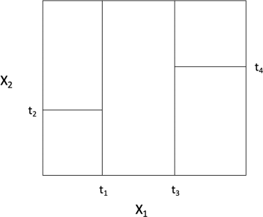
(a) Give an example of a tree classifier on two-dimensional data that gives the following partition of R2 (the outer boundary is not part of the decision boundary). Based on your tree classifier, explain how the first splitting axis and the corresponding splitting point are selected from training data.

(b) Please explain how the boosting algorithm with decision stumps can be used for feature selection (you don’t need to give the details of the boosting algorithm).
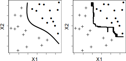
(c) The two images below each show the same dataset, ˜(x) 1 , . . . , ˜(x)n ∈ R2 , and
E(y˜1)ach(..) .i a(n)ge s(∈ {) a(1)cl(})a(e)ti(d)on boundary i(by solid circles)n(a)th(nd)epresp()e(e) t.
the classifier was trained using either a random forest or a kernel support vector machine. Which image do you think should correspond to a classifier trained using a random forest? Please explain your answer.

(d) Assume that you have d features available in your data set. What is a motivation for considering m = ⌊√d⌋ features over m = d features at each split when training a random forest?
Problem 3 (25 points)
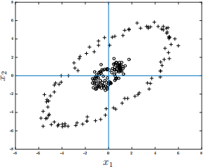
Suppose we want to be able to perform unsupervised classification on the mean-zero data shown in the figure below (the true classes are indicated by ‘o’ and ‘+’), xi ∈ R2 .

We might consider using PCA to find a classification boundary. As a reminder, PCA finds the eigenvectors of the (centered) empirical covariance matrix C = : xixi(T) (note that the data have zero mean). Call the first and second principal components (the eigenvectors) ξ1 ,ξ2 .
(a) (8 points) (Roughly) reproduce the plot of the data and draw the first two principal components. Please label them as ξ1 and ξ2 .
(b) (9 points) Sketch (roughly) the data projected onto the first two principal components, i.e. ⟨x,ξ1 ⟩ and ⟨x,ξ2 ⟩ . (Don’t worry about labeling the tick marks for proper magnitude.)
(c) (8 points) Can we use the principal components to effectively classify the data? In other words, are the classes linearly separable when projected onto the first two principal components? Please explain.
Problem 4 (25 points)
In this problem, we consider regression methods for a data set
D = {(˜(x)1 , ˜(y)1 ), (˜(x)2 , ˜(y)2 ), ··· , (˜(x)n , ˜(y)n )} , (0.1)
where ˜(x)i , ˜(y)i ∈ R for any i ∈ {1, 2, ··· , n} .
(a) (6 points) Suppose that n = 6 and the data set D is given in the following table.
|
˜(x)i |
2.0 |
1.4 |
1.5 |
2.5 |
4.0 |
1.2 |
|
˜(y)i |
11.5 |
12.2 |
10.1 |
14.1 |
10.1 |
19.4 |
We want to fit a least-squares linear regression to this data set (so D is the training data set). Explain how you would obtain the least-squares solution: Please write down relevant matrices/vectors explicitly and state how you would obtain the least-squares solution from them; you are not required to compute the numerical value of the least-squares solution.
Below we consider a different regression method called k-nearest neighbor (kNN) regression. Given a positive integer parameter k and any data set
D′ = {(x1(′), y 1(′)), ··· , (xm(′), ym(′))} ,
a k-nearest neighbor regression trained on D′ has regression function f(x;k, D′ ) : R → R (where x is the feature of an observation and f(x;k, D′ ) is its predicted outcome) that is computed as follows:
1. Find the k points in {x′1, · · ·, x′m} that are closest to xin terms of Euclidean distance d(x, x′i) = |x−x ′ i |. Let ηk(x; D′ ) be the set of indices i ∈ {1, · · · , m} that correspond to those points (that is, x ′ i is among the k points closest to x).
2. Then we assign f(x;k, D′ ) = : yi(′) . That is, f(x;k, D′ ) is the
i ∈ηk (x,D′ )
average of those yi(′) with i ∈ ηk (x;D′ ).
For example, suppose D′ = D is the data set in (a). For k = 3 and x = 2.1, the 3 points that are closest to x are ˜(x)1 = 2.0, ˜(x)3 = 1.5, ˜(x)4 = 2.5 (so ηk (x;D) = {1, 3, 4}). The regression function f(x;3, D) is then the average of y1(′) = 11.5, y3(′) = 10.1, y4(′) = 14.1, that is,
f(x;3, D) = 3/1 (11.5 + 10.1 + 14.1) = 11.9.
(b) (6 points) Assume that n = 6 and D is given as in (a). What is f(x;2, D) and f(x;4, D) for x = 1.4?
(c) For this part, we consider a general data set D as in (0.1) and use the squared-error loss function.
Hint 1 for (c): Note that k controls the model complexity.
Hint 2 for (c): You may adapt the intuitions and ideas for classifiers here (note that the 0−1 loss for classifiers is replaced by the squared-error loss for regression methods here).
(i) (6 points) Suppose that we train a k-nearest neighbor regression on the data set D and assess its performance on a separate test data set. As k increases, how would you expect the training error and test error to change? Please explain.
(ii) (7 points) Please describe a step-by-step procedure to choose an optimal value for the parameter k out of the values {1, 3, 5, 7, 9}, using the data set D.