CSE 250a. Assignment 5

5.1 Gradient-based learning

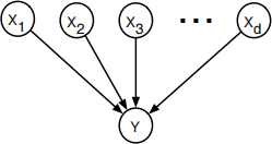
Consider the belief network shown above with binary random variable Y ∈ {0, 1} and conditional proba-bility table (CPT):

Here, we assume that the weights wi ∈ ℜ are real-valued parameters to be estimated from data and that g :ℜ → [0, 1] is a differentiable function that maps its real-valued argument to the unit interval.

Consider a data set of i.i.d. examples  where  = (x1t , x2t , . . . , xdt) denotes the observed vector of values from the t th example for the network’s inputs. Also, as shorthand, let pt = P (Y = 1|).

(a) Show that the gradient of the conditional log-likelihood L = P t log P(yt |) is given by:

where g ′ (z) denotes the first derivative of g(z). Intuitively, this result shows that the differences be-tween observed values yt and predictions pt appear as error signals for learning.

(b) Show that the general result in part (a) reduces to the result in lecture when g(z) = [1 + e −z ] −1 is the sigmoid function.

5.2 Multinomial logistic regression

A simple generalization of logistic regression is to predict a discrete (but non-binary) label y ∈ {1, 2, . . . , k} from a real-valued vector ⃗x ∈ Rd . Here k is the number of classes. For the belief network shown above, consider the following parameterized conditional probability table (CPT):

Consider a data set of T examples , which you can assume to be identically, independently

Also, let pit ∈ [0, 1] denote the conditional probability that the model classifies the tth example by the ith possible label:

The weight vectors can be obtained by maximum likelihood estimation using gradient ascent. Show that the gradient of the conditional log-likelihood  is given by:

Again, this result shows that the differences between observed values yit and predictions pit appear as error signals for learning.

5.3 Convergence of gradient descent

One way to gain intuition for gradient descent is to analyze its behavior in simple settings. For a one-dimensional function g(x) over the real line, gradient descent takes the form:

(a) Consider minimizing the function  by gradient descent, where α>0. (In this case, we know that the minimum occurs at x = x∗; our goal is to analyze the rate of convergence to this minimum.) Derive an expression for the error εn = xn − x∗ at the n th iteration in terms of the initial error ε0 and the step size η >0.

(b) For what values of the step size η does the update rule converge to the minimum at x∗? What step size leads to the fastest convergence, and how is it related to g ′′(xn)?

In practice, the gradient descent learning rule is often modified to dampen oscillations at the end of the learning procedure. A common variant of gradient descent involves adding a so-called momentum term:

where β >0. Intuitively, the name arises because the optimization continues of its own momentum (stepping in the same direction as its previous update) even when the gradient vanishes. In one dimension, this learning rule simplifies to:

xn+1 = xn − ηg′ (xn) + β(xn−xn−1).

(c) Consider minimizing the quadratic function in part (a) by gradient descent with a momentum term. Again, let εn =xn − x∗ denote the error at the nth iteration. Show that the error in this case satisfies the recursion relation:

εn+1 = (1 − αη + β)εn − βεn−1.

(d) Suppose that the second derivative g ′′(x ∗ ) is given by α = 1, the learning rate by η = 4/9 , and the momentum parameter by β = 1/9 . Show that one solution to the recursion in part (c) is given by:

εn = λn ε0,

where ε0 is the initial error and λ is a numerical constant to be determined. (Other solutions are also possible, depending on the way that the momentum term is defined at time t = 0; do not concern yourself with this.) How does this rate of convergence compare to that of gradient descent with the same learning rate (η = 4/9 ) but no momentum parameter (β = 0)?

5.4 Handwritten digit classification

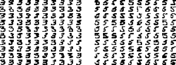
In this problem, you will use logistic regression to classify images of handwritten digits. From the course web site, download the files train3.txt, test3.txt, train5.txt, and test5.txt. These files contain data for binary images of handwritten digits. Each image is an 8x8 bitmap represented in the files by one line of text. Some of the examples are shown in the following figure.

(a) Training

Perform a logistic regression (using gradient ascent or Newton’s method) on the images in files train3.txt and train5.txt. Indicate clearly the algorithm used, and provide evidence that it has converged (or nearly converged) by plotting or printing out the log-likelihood on several itera-tions of the algorithm, as well as the percent error rate on the images in these files. Also, print out the 64 elements of your solution for the weight vector as an 8x8 matrix.

(b) Testing

Use the model learned in part (a) to label the images in the files test3.txt and test5.txt.

Report your percent error rate on these images.

(c) Source code

Turn in a print-out of your source code. Once again, you may program in the language of your choice. You should write your own routines for computing the model’s log-likelihood, gradient, and/or Hessian, as well as for updating its weight vector.