COMPUTER SCIENCE
ECMM461
High Performance Computing
Continuous Assessment 1
Date Set: 9 February 2024
Date Due: 28 February 2024
Return Date: 20 March 2024
1 The Atmospheric Boundary Layer
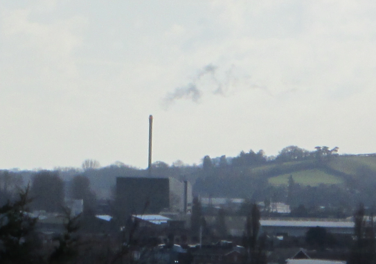
The part of the Earth’s atmosphere nearest the surface is known as the “Atmospheric Boundary Layer”, and in this part of the atmosphere the wind speed increases with height. This causes material emitted from a chimney to be advected at di↵erent horizontal speeds depending on its height. Figure 1 shows material from a chimney being advected by the wind.

Figure 1: Material emitted from a chimney being advected by a horizontal wind
The wind in the Atmospheric Boundary Layer can be approximated as a horizontal velocity which depends only on height (z) and zero vertical velocity. The horizontal velocity as a function of height vx(z) can be represented by a logarithmic profile

where u⇤ is a parameter called the “friction velocity”, z0 is a parameter called the “roughness length”, and k = 0.41 is a constant called Von K´arm´an’s constant.
2 The assignment
In this assignment you will calculate a numerical solution to the advection equation to simulate the movement of a cloud of material in the atmospheric boundary layer. There are four parts to this assignment:
• Task 1: For the first part of this assignment you will parallelise a program which calculates a numerical solution to the 2D advection equation. You have been provided with the program and you will need to parallelise it using OpenMP. This part of the assignment is described in section 2.1.
• Task 2: For the second part of this assignment you will modify the program to change the parameters of the test problem into a more realistic configuration. This is described in section 2.2.
• Task 3: For the third part of this assignment you will add a logarithmic velocity profile to the program. This is described in section 2.3.
• Task 4: For the fourth part of the assignment you will calculate the horizontal profile of the advected material by calculating a vertical average. This is described in section 2.4.
This assignment assesses the following Intended Learning Outcomes:
• Demonstrate skills in parallel processing algorithm design and the practical implementation of such algorithms
• Demonstrate an awareness of numerical e↵ects and the influence of floating point number representation in high-performance computing applications.
• Interpret an informal requirement specification
• Systematically analyse information and make appropriate design choices
2.1 Task 1: Parallelising the program
The advection equation for a two-dimensional scalar field u(x, y) is

where vx and vy are the velocities in the x and y direction respectively. You have been provided with a C program which calculates a numerical solution to the advection equation for a two-dimensional scalar field u(x, y) using finite di↵erence approximations. The program uses one-sided differences to calculate the spatial derivatives

where ui,j is the value of the scalar field u(x, y) at grid point (i, j), dx is the spacing of grid points in the x direction and dy is the spacing of grid points in the y direction. The solution starts from specified initial conditions at time t = 0 and is updated from time t to time t + ∆t using forward-Euler time steps

x The program uses 1000 ⇥ 1000 grid points covering a unit square computational domain 0 ≤ x ≤ 1.0 and 0 ≤ y ≤ 1.0. The initial conditions are a Gaussian given by the expression

The Gaussian is centred at x0 = 0.1, y0 = 0.1 and has a width σx = σy = 0.03. The boundary conditions are u = 0 on all boundaries. The program calculates 1500 time steps, and the time step size is calculated from the Courant condition with a CFL number of 0.9. The velocities in the x and y directions are vx = 0.01 and vy = 0.01 respectively.
The first part of the assignment is to parallelise the program provided using OpenMP. There are 10 loops or loop nests (a loop over j inside a loop over i) in the program and these have been identified with a comment of the form
/* LOOP N */
where N is an integer between 1 and 10 inclusive. For each loop or loop nest you should decide whether it can be correctly parallelised by adding an OpenMP directive:
• If the loop can be correctly parallelised then you should parallelise it by adding an OpenMP directive, ensuring that all variables are correctly scoped. You do not need to scope variables which have the const qualifier.
• If the loop cannot be parallelised then you should add a comment in the program to say that the loop cannot be parallelised and explain why.
To build the serial program on a Lovelace lab PC use the command
gcc -o advection2D -std=c99 advection2D.c -lm
To build the program on a Lovelace lab PC with OpenMP enabled use the command
gcc -fopenmp -o advection2D -std=c99 advection2D.c -lm
A gnuplot script which plot the final values of u(x, y) has been provided.
The parallelised version of the program must produce exactly the same output as the original program.
2.2 Task 2: Modifying the calculation
In this section you will modify the example program to change the test problem so that it more closely resembles a cloud of material emitted from a chimney. The calculation will represent ma-terial advecting into the computational domain from the left hand side by specifying a boundary condition which varies with height and varies over time. Modifying the calculation requires chang-ing the size of the computational domain, the initial conditions, one of the boundary conditions, the velocities and the number of time steps. In the following instructions distances are measured in metres (m), time in seconds (s) and velocities in metres per second (m/s).
• The test problem uses a computational domain which is a unit square (it covers the range 0 ≤ x ≤ 1.0 and 0 ≤ y ≤ 1.0). Change the computational domain so that it covers the range 0 ≤ x ≤ 30.0 m and 0 ≤ y ≤ 30.0 m.
• The calculation will start with an empty computational domain. Change the initial conditions so that u(x, y) = 0 everywhere.
• Modify the boundary condition at x = 0 (the left boundary) so that it varies with height (y) and time (t) according to the following equation:

Set the values of the parameters to y0 = 15.0 m, σy = 5.0 m, t0 = 3.0 s, σt = 1.0 s
• The material in the atmospheric boundary layer advects horizontally but not vertically. In this part of the assignment you will test the calculation with a constant horizontal velocity of 1.0 m/s. Change change the horizontal velocity to vx = 1.0 m/s and change the vertical velocity to vy = 0.
• Change the maximum number of time steps to 1000 so that the material does not advect out of the computational domain.
After you have made these changes re-compile and re-run the program. If necessary update the OpenMP directives to ensure that the program produces identical results with and without OpenMP.
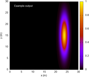
Now plot the final values of u(x, y). The final values are in the file final.dat. If you are using the example gnuplot script you will need to change the axis limits to match the new computational domain size. A plots of the final values of u(x, y) is shown in figure 2 for comparison.

Figure 2: Final values of u(x, y) from the calculation in section 2.2
2.3 Task 3: Adding vertical shear
In this section you will modify the program so that the horizontal velocity varies with height according to the logarithmic profile given in equation 1. The logarithmic profile should only be used if z is greater than the roughness length z0. If z>z0 calculate the horizontal velocity using equation 1, and if z > z0 set the horizontal velocity to zero. The parameters of the profile should be set to u⇤ = 0.1 m/s, z0 = 1.0 m and k = 0.41.
In the program the variable y represents the height z in equation 1. The computational domain, the initial conditions and the number of time steps should be kept at the values specified in the previous section (section 2.2).
Modify the horizontal velocity as described above and re-run the program. If necessary update the OpenMP directives to ensure that the program produces identical results with and without OpenMP.
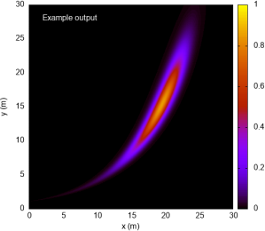
Now plot the final values of u(x, y). Plots of the final values of u(x, y) are shown in figure 3.

Figure 3: Final values of u(x, y) from the calculation in section 2.3
2.4 Task 4: Calculating the vertically averaged distribution
In this last section you should calculate the vertically averaged distribution of u(x, y) at the end of the calculation in section 2.3. The vertical average should cover the whole vertical domain but should not include the boundary values. The code you add to the program does not need to be parallelised. Plot the vertically averaged values of u as a function of x using a line graph.
3 Deliverables
The deliverables for this assignment are the source code for the program with your modifications, and the three plots showing your results:
1. Source code for the final version of the program. The program should include the OpenMP directives added in section 2.1 with any changes required to ensure the modified program continues to work correctly. The computational domain, the initial conditions, the velocities and the number of time steps should be set to the values used in section 2.3.
2. Three plots showing the output from running the program. The required plots are:
• A plot of the final values of u(x, y) from section 2.2
• A plot of the final values of u(x, y) from section 2.3
• A plot showing the vertically averaged profile of u from section 2.4
The plots may be generated using the gnuplot script provided, or alternative plotting software of your choice provided the data values in the plot are clearly represented. Your plots should be delivered as PNG or PDF files.
The deliverables should uploaded to ELE a single zip or tar file containing the source code for the final version of the program, and the four plots. The deadline for submission is 12 noon 28 February 2024.
4 Mark scheme
A total of 100 marks are available for this assignment:
1. Task 1: Parallelising the program (30 marks)
(a) For each of the 10 loops or loop nests identified in the program there are two marks to be awarded according to the following criteria:
• The loop has been correctly identified as either one that can be parallelised or one that cannot be parallelised (1 mark)
• If the loop can be parallelised then an appropriate OpenMP directive has been added which unambiguously and correctly scopes all variables. Variables with the const qualifier do not need to be scoped (1 mark)
OR
• If the loop cannot be parallelised then a comment has been added with a correct explanation of why the loop cannot be parallelised (1 mark).
(b) An additional 10 marks are awarded if the parallelised program produces results which exactly match the original serial program.
2. Task 2: Modifying the calculation (20 marks)
15 marks are awarded for correctly modifying the computational domain, the initial con-ditions, the boundary condition at x = 0 and the number of time steps, as specified in section 2.2. 5 marks are awarded for the plot of the final results.
3. Task 3: Adding vertical shear (25 marks)
20 marks are awarded for correctly modifying the velocity profile as specified in section 2.3. 5 marks are awarded for the plot of the final results.
4. Task 4: Calculating the vertically averaged distribution (25 marks)
20 marks are awarded for correctly modifying the program to calculate the vertically averaged distribution of u, as specified in section 2.4. 5 marks are awarded for the plot of the final results.